


The challenge of language
Every day, millions of people use language models like ChatGPT to write emails, brainstorm ideas, get help with coding, or just have a conversation. It’s hard to imagine that just a few decades ago, machines struggled with even the simplest language tasks. Have you ever wondered how these powerful tools actually work? What challenges did researchers face in achieving the level of language understanding found in current large language models (LLMs)?
To understand that journey, we must go back more than seventy years to a question posed by Alan Turing in his 1950 paper, "Computing Machinery and Intelligence": Can machines think? This paper introduced ideas that would eventually become the foundation of what we now think of as artificial intelligence (AI). Back then, computers were large, slow, and accessible only to a small percentage of the population. However, Turing’s question raised an interesting vision: machines that could understand and use human language like we do. Early AI and natural language processing (NLP) researchers dreamed of building systems that could chat, translate, and reason like humans. This vision set the groundwork for the development of NLP, inspiring the following research that led to the technologies we use today.
Early NLP systems relied on hand-crafted rules and grammar-based approaches. The goal was to model language in a structured, logical way (much like how a linguist or logician would break down a sentence). These approaches allowed computers to parse and analyze text according to predefined grammatical rules, enabling tasks such as syntactic parsing, part-of-speech tagging, and basic question answering.
One of the earliest and most iconic examples of general-purpose systems is Eliza, often considered the first chatbot capable of processing natural language. Developed in 1964 at MIT by Joseph Weizenbaum, Eliza was designed to simulate a therapist by mimicking the conversational style of a Rogerian psychotherapist. Eliza worked using simple pattern matching and substitution rules to generate responses that sounded conversational, though it actually had no real understanding of the content. For example, a pattern as follows was defined:
Pattern: I feel X.
Eliza's response: Why do you feel X?
So if a user typed “I feel sad”, the interaction would look like this:
User input: I feel sad
Eliza's response: Why do you feel sad?
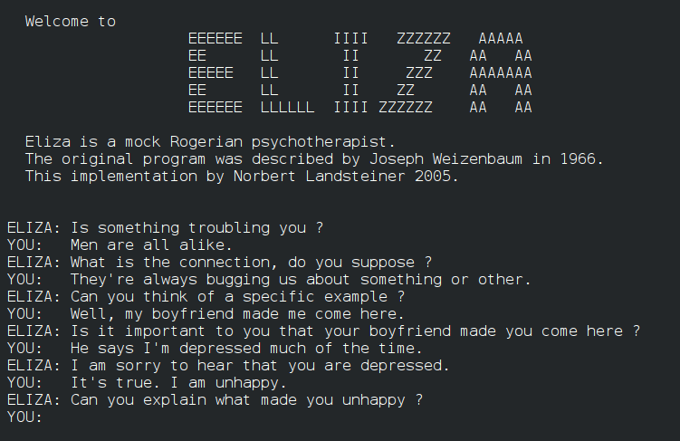
While Eliza was limited in its capabilities, it marked an early attempt to simulate meaningful conversation. It highlighted both the potential and the challenges of building systems that could appear to understand language.
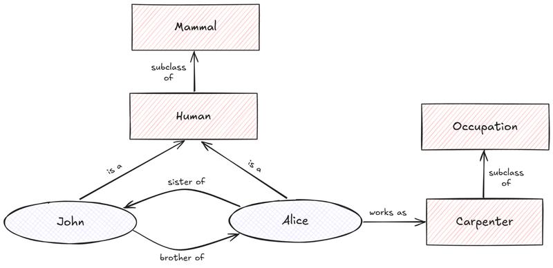
As researchers moved beyond simple pattern matching, they began exploring more structured ways to represent knowledge and meaning through ontologies and semantic networks. While a deep dive into ontologies is beyond the scope of this blog post, they can be thought of as formal frameworks that define concepts and the relationships between them. This enables machines to better comprehend context and meaning in a manner that extends beyond simple word patterns. They can capture relationships within a specific domain (like sports) or across general knowledge.
While the NLP techniques we have explored worked reasonably well in narrow domains, they didn’t scale effectively to more general problems. The need to define these handcrafted rules was very labor-intensive and also really brittle due to the nature of language. These limitations, along with unmet expectations, led to a decline in enthusiasm and reduced funding, starting a period known as the AI winter.
Learning from data: Moving beyond rules
In the late 80s, statistical approaches to NLP began gaining traction, mainly due to the increasing availability of digital corpora and advances in computational power. Researchers no longer tried to define language through handcrafted rules. Instead, language was modeled as a sequence of random variables, where we estimate how likely it is for one word to follow another, based on past examples from real-world data. This core idea still underlies modern large language models, but with some refinements.
N-grams are one of the fundamental building blocks of early statistical language modeling. The idea is straightforward: given a sequence of words, what’s the probability of the next word? To answer that, n-gram models make a simplifying assumption: a word depends only on the few words that came right before it. This is known as the Markov assumption. So, for example:
- A bigram model (n=2) assumes that the probability of each word depends only on the one immediately before it.
- A trigram model (n=3) considers the previous two words.
And so on for larger values of n. These models allow us to estimate probabilities like:
P(tennis|I like)
Or, in other words, what is the probability of “tennis” being the following word after “I like”? This probability is computed by considering all the corpora that were fed to the model, and counting how many times the word "tennis" appears after the phrase "I like". The larger the value of n, the more context we are adding to compute these probabilities, but also the more data we would need for these estimates to be reliable. N-gram models were extremely useful in early NLP applications such as text autocompletion, spelling correction, and information retrieval.
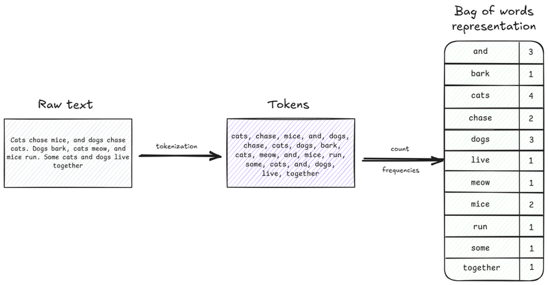
Another major advancement during this time was the development of ways to represent text in a format that statistical models could easily process. One of the earliest and most influential methods was the bag-of-words model. It works by treating a piece of text as a “bag” of the words it contains, without caring about grammar and their order. The model simply counts how many times each word occurs, turning the text into a numerical vector of word frequencies. This made it easier for computers to analyze and compare texts based on their vocabulary.
There were a lot of other interesting developments during this time that built on the basic ideas of n-grams and bag of words. One of them was Term Frequency-Inverse Document Frequency (TF-IDF), which improved the bag of words approach by not only counting how often a word appears, but also the importance of that word within the text.
These representations also made it easier to apply machine learning (ML) techniques to language. For example, Support Vector Machines (SVMs) became popular for tasks like spam detection or sentiment analysis. These models took the word counts or TF-IDF scores and learned how to sort texts into categories (like whether an email is spam or not) based on patterns in the data.
Going deeper into these techniques and others that appeared during this time would require their own dedicated posts or articles. For now, the key takeaway is that this era marked a shift from handcrafted rules to learning from data. It was a huge step forward, and it helped computers get better at dealing with language in more flexible and effective ways. But these methods still had their limitations, which led researchers to explore new approaches that led to LLMs. We’ll look at the most influential techniques next.
Capturing semantic meaning
While previous approaches were a huge step forward, they still missed some important pieces for deeper language understanding and reasoning.
One of the key limitations was that these models couldn’t capture semantic similarity between words. For example, words like Madrid and Paris are both related to the same concept (cities, and more concretely, capitals), so they are likely to behave similarly in a sentence. However, earlier models treated them as completely unrelated words. This began to change in the early 2000s, when Yoshua Bengio introduced the idea of distributed representations. This would later evolve into what we now refer to as word embeddings.
At a high level, word embeddings are just another way of encoding words so they can be processed by a computer. Word embeddings represent each word as a dense vector: a list of numbers, where each dimension captures something about the word’s meaning. Unlike the bag-of-words model, where the number of dimensions equals the size of the vocabulary, the number of dimensions of word embeddings is much smaller and can be adjusted to suit different tasks. For example, we could represent the word Paris as follows:
Paris = [0.177, 0.385, -0.926]
While the vector representation of a word might not look very impressive on its own, what makes word embeddings powerful is how they are learned: words that appear in similar contexts end up close together in the vector space. In other words, these vectors capture semantic similarity, so words like Paris and Madrid, or doctor and nurse, will have embeddings that are near each other. The following image, where we plot real-word embeddings in a two-dimensional space, can help visualize this idea more clearly.
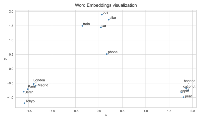
We can see how word embeddings of capital cities are grouped in the bottom left corner. That is, their word embedding (distributed representation) is similar. A model that is fed these word embeddings will associate Madrid and London as similar words. We can find similar groupings for fruits and means of transportation in the visualization.
Word embeddings also allow us to use arithmetic to learn facts about the world. For example, we can leverage the word embeddings that we have for Paris, France, and Germany to derive that the capital of Germany is Berlin. These analogies aren’t perfect, but they work surprisingly well and show that embeddings capture more than just similarity: they encode relationships between words. So, at this point, researchers found a way to represent words in a way that captures meaning, similarity, and even basic analogies. All of this makes word embeddings incredibly useful for natural language processing tasks. But this raises a natural question: how are these word vectors actually learned?
In most cases, word embeddings are learned using a type of neural network. While diving into the details of neural networks is beyond the scope of this post, we can think of them (at least at a high level) as systems that perform matrix operations. You feed in a vector (like a one-hot representation of a word), apply a set of matrix multiplications using learned weights, and get back another vector.
If we go back to our previous example, we could imagine a neural network trained to determine whether a word refers to a capital city. This network might take in a word as input, run it through a few internal layers, and output a probability. So, for example, 0.92 for “Paris” (likely a capital) and 0.03 for “cat” (very unlikely).
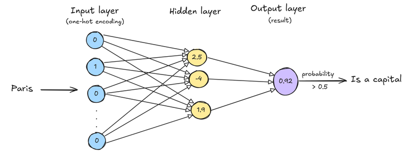
To train this model, we would feed it examples along with expected outcomes (telling it that “Paris” should return a high probability, while “cat” should return a low one). The network then updates its internal weights to better align its outputs with these targets. After training, we can input a new word like “Berlin” and the network would correctly identify it as another capital city.
Now, here’s where embeddings come in: while classification is the model’s main goal, it turns out that the hidden layer contains a very useful representation of each word. That is, researchers found that the values in this hidden layer capture semantic information. For example, “Paris,” “Berlin,” and “Madrid” might end up with similar internal representations because they often appear in similar contexts. These internal representations are the actual word embeddings.
While the main idea of distributed representations was introduced in the early 2000s, it was not until 2013 that they became widely adopted and used, with the release of Word2Vec by Google. Word2Vec is a toolkit that allows the training and use of pre-trained (i.e., pre-computed and ready to be used) word embeddings. Soon after, researchers and companies began releasing pre-trained word embeddings, trained on everything from news articles to Wikipedia, so they could be used by other people for their natural language processing tasks.
Most NLP tasks saw significant performance improvements once word embeddings replaced earlier encoding methods like bag of words or TF-IDF. By capturing the semantic relationships between words, embeddings helped models generalize better across language. Some specific tasks were particularly well-suited for this kind of representation and achieved great results (even by today’s standards!). These include paraphrase detection, named entity recognition, sentiment analysis, and topic modeling, among others.
Conclusion
In this first part, we explored the shift from early hand-crafted approaches to statistical methods to build intelligent systems. This shift, from explicitly modeling language ourselves to instead giving large corpora to computers so they can extract patterns and learn from them, has been the basis of most NLP systems over the past decades. Word embeddings took this one step further, allowing computers to capture the semantic meaning of words and relationships between them. These chapters have laid the foundation needed to understand modern NLP systems and LLMs. In the next part, we will explore the final two ingredients that led to LLMs and how they truly work.