Autoencoders 101: Learning hidden patterns in your data

Introduction

Autoencoders are a powerful unsupervised learning tool for extracting meaningful data representations by reconstructing input through neural networks. They are used in various applications, from denoising to generative modeling, and are foundational for modern AI systems like Midjourney. This blog post will explore autoencoders in depth, covering their structure, training, types, and applications. We’ll also compare them with traditional methods to help you determine when to use them. Finally, we'll provide a hands-on example: building a denoising autoencoder with TensorFlow and the STL-10 dataset to demonstrate its practical power. By the end, you'll have a strong conceptual and practical understanding, plus a ready-to-use implementation.

Necessary concepts

To understand this blog post, we suggest a basic understanding of neural networks and their inner workings, as we won’t go into the details of these for the sake of conciseness. Below we have a list of curated resources with the topics that are foundational to understanding autoencoders.

• What is a neural network?
• The spelled-out intro to neural networks and backpropagation: building micrograd
• What is Loss Function?
• Convolutional Neural Networks: A Comprehensive Guide

What are Autoencoders?

At their core, autoencoders are a type of neural network that’s trained to reconstruct its input; in other words, they take in some data, process it, and then try to output the same data. While this might sound trivial, the interesting part is the middle - called the Latent Space - which is a smaller representation with the most defining features of our data. This forces the model to capture the most essential features of the input, effectively learning a compressed version of it.

Structure of autoencoders

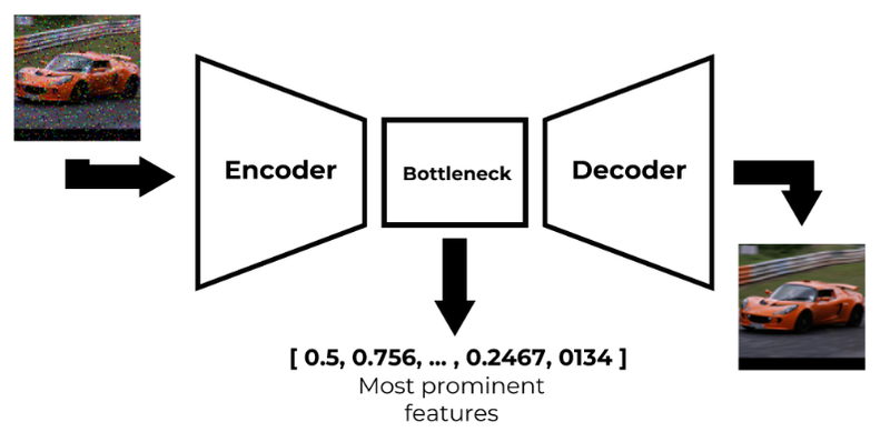
The high-level architecture of an autoencoder (image by author)

A typical autoencoder consists of three main components:

1. The Encoder: This part of the network takes the high-dimensional input data and compresses it into a lower-dimensional representation. It essentially maps the input to the latent space using a series of learnable transformations.
2. Bottleneck (Latent Space): This is the most compressed version of the input. It's a distilled representation that ideally captures the most informative features of the data while discarding noise or redundancy.
3. Decoder: The decoder takes the compressed representation and attempts to reconstruct the original input as closely as possible. It performs the inverse operation of the encoder.

How are autoencoders trained?

Training an autoencoder is an unsupervised process where the model learns to reconstruct its input as accurately as possible. Despite having a neural network architecture, autoencoders don’t require labeled data — the input itself serves as the target output.

The training process begins with an input x, which passes through the encoder network to produce a latent representation z. This compressed representation is then passed through the decoder to produce a reconstruction x2. The network is trained to minimize the difference between the original input and its reconstruction. This is done using a loss function such as Mean Squared Error (MSE) or Binary Cross-Entropy (BCE), depending on the nature of the data.

For example, in image reconstruction tasks with normalized pixel values between 0 and 1 (such as black and white images in MNIST), BCE is commonly used. For other continuous-valued data (such as colored images in STL-10), MSE is often the preferred choice. The goal is to minimize the reconstruction loss across all input samples, encouraging the network to learn compact, informative representations in the latent space.

At each step, a batch of input data is passed through the encoder and decoder. The reconstruction loss is computed, gradients are calculated via backpropagation, and the parameters are updated to reduce the loss.

Techniques to prevent overfitting in autoencoders

It's important to prevent overfitting in autoencoders, as without proper constraints, they may simply learn to copy the input directly to the output. This behavior defeats the purpose of learning a meaningful, compressed representation in the latent space. To encourage the model to generalize and capture essential features of the data, several common techniques can be applied, such as:

• Using dropout layers: Dropout involves randomly deactivating a subset of neurons during training. This forces the autoencoder to learn robust, general features rather than relying on specific activations, reducing the risk of overfitting.

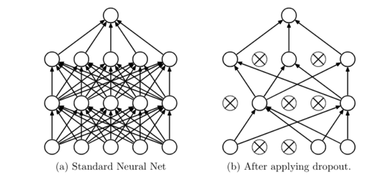
Visualization of using dropout layers (Taken from Dropout: A Simple Way to Prevent Neural Networks from Overfitting by Nitish & et al.)

• Reducing the size of the latent space: By constraining the dimensionality of the latent representation, we force the model to capture only the most essential features necessary for reconstructing the input. A smaller latent space limits the model's capacity to memorize fine-grained details, encouraging abstraction.
• Applying data augmentation techniques: This involves introducing variations of the input data, such as flipping, rotating, scaling, or adding noise. These variations increase the diversity of the training set, helping the model to generalize better by learning to reconstruct data under slightly different conditions.

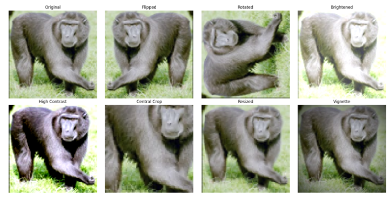
Data augmentation examples (image by author)

These techniques, when used appropriately, encourage the autoencoder to learn meaningful and compressed representations of the data, leading to better generalization and performance on unseen inputs.

Usage and types of Autoencoders

Autoencoders are pretty flexible, having multiple usages and types to choose from depending on the task. Despite the simplicity of their architecture, they can be adapted for various tasks by modifying how they learn and what they're optimized to do. The types of autoencoders are the following:

1. Vanilla Autoencoder: It is used for dimensionality reduction and data compression. It’s the simplest form of autoencoder, with a symmetrical encoder-decoder structure and a bottleneck layer in between. Its goal is to reconstruct the input data as faithfully as possible, thereby learning compressed representations. With this autoencoder, you could, for example, compress high-dimensional sensor data into fewer dimensions for visualization or storage.
2. Denoising Autoencoder: It’s made for noise reduction and data cleaning. In this variant, noise is intentionally added to the input data, and the model is trained to reconstruct the original, clean version. This encourages the model to learn more robust features and ignore noise. As an example, this autoencoder can be applied to the removal of watermarks from images.
3. Sparse Autoencoder: This type of autoencoder is used in feature extraction and anomaly detection. It adds a sparsity constraint to the latent space, forcing most of the neurons in the bottleneck layer to remain inactive, leading to more interpretable features. It’s especially useful when we want the model to learn high-level, abstract representations. An example use case would be extracting key features from customer behavior data for identifying unusual spending patterns.
4. Variational Autoencoder: It’s used for generative modeling and probabilistic representation learning. They don’t just learn a fixed latent representation - they learn a distribution over the latent space. This allows them to generate new data points by sampling from this distribution, making them powerful tools for generative tasks like image synthesis or data augmentation. You could use them to generate new, realistic human faces from a dataset of already existing faces.
5. Contractive Autoencoder: This autoencoder focuses on learning robust representations. It adds a penalty to the loss function that constrains the model to be less sensitive to small input variations. The goal is to learn stable representations that don’t change drastically with minor perturbations, which is useful for learning meaningful data manifolds. This could be applied, for example, in identifying if a person's signature is valid, even while using different pens, speeds, and pressures.
6. Convolutional Autoencoder: used for image compression and image generation. It’s designed specifically for image data, and convolutional autoencoders replace the fully connected layers with convolutional layers. These models capture spatial hierarchies in data more effectively and scale better with larger input dimensions. You can use this to generate a greater resolution representation of a low-resolution image.
7. Sequence-to-Sequence Autoencoder: they’re used for time series data, language modeling, and general sequences, as the name suggests. They encode a sequence of data into a fixed-length vector representation to later down the line reconstruct this sequence. You could apply it, for example, to encode customer session data in web analytics.

When is an autoencoder the right fit for your application?

Autoencoders excel with complex, high-dimensional data where non-linear patterns are suspected, particularly for images, audio, or time series. They're ideal when a compact internal representation, data reconstruction, or generation is needed, often outperforming classic methods for denoising or compression.

Even though autoencoders are powerful for uncovering hidden structures, non-linear dimensionality reduction, and intelligent data cleaning or generation, they are computationally intensive, less interpretable, and prone to overfitting without proper regularization. They perform poorly on small datasets and are often overkill for simple, low-dimensional, or linearly separable data, where something like Principal Component Analysis (PCA) or other simpler methods are more appropriate. Ultimately, as with everything in software, the choice depends on project scale, complexity, and goals.

Practical example - Denoising Autoencoder on STL-10

To bring all the theory into practice, let's walk through a real-world implementation of a denoising autoencoder using the STL-10 dataset. STL-10 is a dataset of 96x96 color images, often used for unsupervised and self-supervised learning benchmarks. In our example, we’ll intentionally add noise to the images and train an autoencoder to recover their clean versions. You can find the full code for this project on our GitHub.

We begin by loading and preprocessing the dataset. To keep things efficient, we use only the unlabelled portion of STL-10, normalize the image pixel values to the range [0, 1], and introduce random Gaussian noise. If the data has already been processed and saved, we simply load it from disk, which allows us to save time for repeated runs.

The autoencoder itself is built using TensorFlow and Keras. Its architecture follows an encoder-decoder structure with skip connections that help preserve finer details during reconstruction. The encoder uses a series of convolutional layers and pooling operations to compress the image into a smaller latent representation. The decoder then uses upsampling and convolution to reconstruct the original image, gradually bringing it back to the original resolution. To help the model keep important details, skip connections are used. These connections pass information directly from the encoder to the decoder, making it easier for the model to reconstruct clear and accurate images.

To train the model, we use MSE as the loss function, which, as mentioned above, helps get the correct details in our multi-channel pixel data. If a trained model already exists, it is loaded; otherwise, training is run for 50 epochs with a batch size of 128.

Once training is complete, we visualize the model’s performance by comparing original, noisy, and denoised images side by side. The results clearly show that the autoencoder successfully learns to remove the noise and recover fine details in many of the images, even though it was never shown clean images during inference.

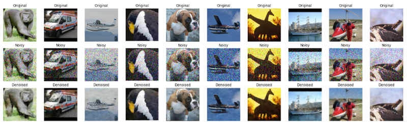
Results obtained by running the code (image by author)

Conclusion

Autoencoders are a foundational concept in deep learning that goes far beyond simple reconstruction. As we’ve explored in this post, they offer a powerful and flexible framework for learning meaningful representations from unlabeled data. They work whether your goal is to compress, denoise, detect anomalies, or even generate new samples.

Through our hands-on example using the STL-10 dataset, we saw how a denoising autoencoder can learn to clean noisy images effectively. This practical case illustrated not just how to build and train such a model in TensorFlow, but also how it can generalize and enhance data quality without explicit supervision.

Of course, autoencoders aren’t always the best tool for every situation. Simpler tasks may be better served by traditional techniques like PCA or classical filters. But when the data is complex, unlabeled, and you need to uncover hidden structure, autoencoders truly shine.